

Ask someone familiar with Road Accident Fund quantums what contingency deductions should be applied, and the answer may come quickly:
5% for past loss. 15% for future loss.
Those figures are useful shorthand. But they can also obscure what contingencies are actually intended to do.
The courts have repeatedly recognised that there are no fixed rules governing contingencies.
For example.
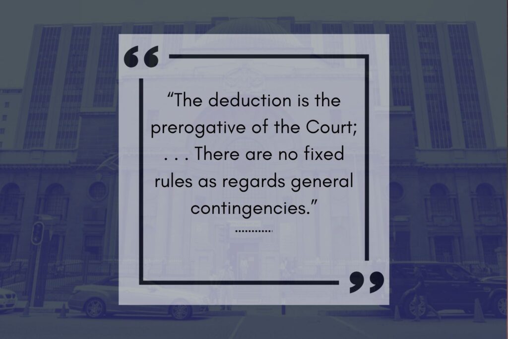
In Road Accident Fund v Guedes (611/04) [2006] ZASCA 19; 2006 (5) SA 583 (SCA), the SCA considered the approach to general contingencies and quoted Koch’s formulation with approval:
“The deduction is the prerogative of the Court; . . . There are no fixed rules as regards general contingencies.”
The familiar percentages are useful benchmarks, but the appropriate deduction ultimately depends on the facts of the particular claimant and the uncertainties inherent in the assumed career paths.
For attorneys dealing with loss-of-earnings claims, the better question is therefore not:
“What is the normal contingency?”
It is:
“What risks and uncertainties actually exist in this claimant’s earnings scenarios — and which of those have not already been reflected in the calculation?”
That is where contingency analysis becomes important.
Contingencies are the bridge between the model and real life
An actuarial calculation necessarily simplifies reality.
It may assume that, but for the accident, a claimant would have progressed through a particular career path, received salary increases, reached a particular earnings level and retired at a particular age.
The actuary can calculate the present value of that projected income.
But real careers rarely develop exactly as modelled.
A claimant might have experienced periods of unemployment, changed occupation, been promoted faster or slower than expected, suffered an unrelated illness or injury, been retrenched, changed employers, retired earlier or later, or experienced favourable career opportunities that could never have been predicted.
Contingencies provide a mechanism through which these “vicissitudes of life” can be recognised.
Importantly, those vicissitudes are not necessarily negative. Life can produce favourable as well as adverse outcomes. A contingency exercise is therefore not simply an exercise in finding reasons to reduce a claimant’s claim.
It is an assessment of uncertainty.
The actuarial calculation is not the final answer
This distinction is fundamental.
The actuary calculates the financial consequences of a set of assumptions. The court ultimately determines what is fair and reasonable.
The classic authority remains Southern Insurance Association Ltd v Bailey NO, where the Appellate Division recognised actuarial calculations as a useful and logical method of estimating loss while confirming that the assessment of damages ultimately involves judicial discretion.
That distinction remains important in modern RAF litigation.
A contingency is therefore not simply an actuarial input.
It is ultimately a legal conclusion informed by the evidence.
The actuary can illustrate the financial effect of different contingency assumptions. The legal team must establish the evidential basis for why one set of assumptions may be more appropriate than another.
Why 5% and 15% should not become automatic
The familiar 5% past and 15% future deductions remain useful reference points.
They are not rules.
Another frequently referenced approach is the Goodall or “sliding-scale” guideline, broadly allowing approximately half a percentage point for each year remaining to retirement.
Again, however, the purpose of such guidelines is to provide a starting point for the exercise of judgment — not to replace it.
The circumstances of individual claimants differ too significantly for contingency deductions to become mechanical.
Consider the difference between:
- a 55-year-old professional with a stable 30-year employment history and a relatively predictable path to retirement; and
- a 15-year-old learner whose tertiary education, occupation, career progression and lifetime earnings all need to be projected.
Both claims involve future loss.
But the degree of uncertainty contained in those projections is clearly not the same.
The benchmark should therefore be the beginning of the contingency discussion, not the end of it.
Past loss can also contain uncertainty
It is tempting to think of the calculation as:
Past = known.
Future = uncertain.
That is not always correct.
The claimant’s actual post-accident earnings during the past period may be readily ascertainable.
But loss of earnings requires a comparison between what actually happened and what would probably have happened but for the accident.
Even over an historical period, that counterfactual can remain hypothetical.
Would the claimant have been promoted?
Would a young claimant have completed a qualification?
Would a self-employed claimant’s business have continued growing?
Would an unemployed claimant have entered the labour market when suggested by the industrial psychologist?
The calendar may have moved those years into the past. It does not necessarily eliminate the uncertainty surrounding the hypothetical uninjured career.
This is one reason contingency analysis should follow the evidence rather than simply treating “past” as certain and “future” as uncertain.
The real battleground: Differential contingencies
In many RAF matters, the important issue is not the contingency percentage in isolation.
It is the difference between the contingencies applied to the uninjured (pre-morbid) and injured (post-morbid) scenarios.
Consider a claimant who has returned to work and remains employable after the accident.
At first glance, that may suggest limited future loss.
But suppose the evidence indicates that the claimant:
- is now an unequal competitor in the labour market;
- depends on an accommodating employer;
- has fewer promotional opportunities;
- would struggle to obtain equivalent employment if retrenched;
- is more vulnerable to periods of unemployment; or
- faces an increased risk of early retirement.
Simply reducing the injured earnings trajectory may not fully capture those risks.
A higher contingency on the injured earnings scenario can recognise the increased uncertainty surrounding the claimant’s ability to sustain those earnings over the remainder of their working life.
This is commonly referred to as a contingency differential or contingency spread.
And relatively small changes in that spread can have a surprisingly large effect on quantum.
CASE STUDY
Let’s look at an example of contingencies being applied in practice.
Assume the actuarial present values before contingencies are:
Uninjured future earnings: R6,000,000
Injured future earnings: R3,500,000
Same claimant. Same expert assumptions. Same actuarial model.
Now consider three possible contingency scenarios:
| Contingencies: Pre-morbid / Post-morbid |
Uninjured after contingency |
Injured after contingency |
Future Loss |
|---|---|---|---|
| 15% / 15% | R5,100,000 | R2,975,000 | R2,125,000 |
| 15% / 25% | R5,100,000 | R2,625,000 | R2,475,000 |
| 15% / 35% | R5,100,000 | R2,275,000 | R2,825,000 |
The earnings assumptions have not changed.
The uninjured career path has not changed.
The injured career path has not changed.
The actuarial methodology has not changed.
Yet moving the injured contingency from 15% to 35% increases the calculated future loss by R700,000.
That is the practical significance of a contingency differential.
The contingency debate is not merely a debate about percentages. It is a debate about risk - with a direct Rand consequence for quantum.
But beware of double-counting risk
There is another side to this.
A higher contingency should not become a convenient mechanism for reflecting risks that have already been explicitly incorporated into the underlying earnings scenario.
Suppose, for example, that the industrial psychologist has already assumed:
- retirement at 60 rather than 65;
- slower post-accident career progression;
- a lower earnings ceiling; and
- identifiable periods of unemployment.
If the actuarial calculation expressly incorporates those assumptions, applying an additional substantial contingency because of precisely the same risks may effectively count them twice.
This is why one of the most important questions when considering contingencies is:
“What has already been modelled?”
The distinction can be expressed simply:
Scenario assumptions model identifiable risks.
Contingencies accommodate residual uncertainty.
The two should complement one another rather than overlap.
What should attorneys interrogate?
When reviewing an actuarial loss-of-earnings calculation, attorneys should therefore look beyond the final quantum.
1. How speculative is the uninjured career path?
Consider the claimant’s age, education, employment history, career progression and the strength of the evidence supporting the projected career.
The greater the uncertainty in the counterfactual, the more important the contingency analysis becomes.
2. How secure is the injured career path?
Continued employment does not necessarily mean there is no future vulnerability.
The important question may not be:
“Is the claimant currently earning?”
but rather:
“How sustainable are those earnings over the remainder of the claimant’s working life?”
3. Which risks have already been incorporated into the expert assumptions?
Look carefully at early retirement, reduced career progression, lower earnings ceilings, unemployment assumptions and other explicit adjustments.
This helps identify what uncertainty remains to be dealt with through contingencies.
4. What evidence supports the contingency differential?
An elevated post-accident contingency should ideally flow from the evidence.
That may include:
- industrial psychology evidence;
- occupational limitations;
- employment history;
- employer accommodation;
- vulnerability to retrenchment;
- reduced mobility in the labour market; and
- the claimant’s residual earning capacity.
The stronger the evidential foundation, the stronger the contingency argument.
5. What is the Rand value of the contingency dispute?
This question is often overlooked.
A disagreement between, for example, 25% and 35% may sound relatively modest when expressed purely as percentages.
But depending on the underlying earnings values, it may represent hundreds of thousands — or even millions — of Rand in disputed quantum.
Where contingencies are genuinely contentious, attorneys should consider asking the actuary to illustrate alternative scenarios.
Don’t only debate the percentage. Quantify the consequence.
From a single answer to a range of outcomes
This is also why we believe actuarial reports should increasingly help practitioners understand the sensitivity of quantum to different reasonable assumptions.
A single calculated figure can create a false impression of precision.
In reality, the actuarial model may contain several variables over which reasonable experts — and ultimately the parties or the court — may differ.
Contingencies are a particularly good example.
Seeing the effect of alternative assumptions can help attorneys and their legal counsel:
- assess settlement proposals;
- understand the materiality of an expert disagreement;
- prepare for joint minutes;
- identify which assumptions actually matter to quantum; and
- focus negotiations on the issues with the greatest financial consequence.
Vector FastFlex
Model it. Stress it. See the impact.
Vector FastFlex allows attorneys to explore alternative assumptions and immediately see their effect on quantum.
Rather than debating an assumption only in abstract terms, FastFlex helps translate that assumption into its Rand impact.
Because quantum is about more than a number — it is about understanding the range of possibilities.

Contingencies should tell the story of the case
Perhaps the most useful way to think about contingencies is that they are not merely deductions.
They are an expression of risk.
A good actuarial calculation establishes the financial architecture of the claim.
A good contingency analysis then asks how confident we should be that the assumed earnings paths would actually have unfolded.
That analysis should be grounded in the claimant’s evidence — not simply inherited from what was applied in the previous matter.
So while 5% and 15% remain useful reference points, they should never replace the real enquiry:
What uncertainties exist in this particular claimant’s uninjured and injured career paths, which have not already been allowed for, and how should those uncertainties reasonably affect the value of the claim?
That is where actuarial calculation meets legal judgment.
And in many RAF loss-of-earnings matters, it is where a significant part of the quantum is ultimately determined.
#VectorActuaries #RAFClaims #Contingencies #LossOfEarnings #ActuarialReports #Quantum #RoadAccidentFund #PersonalInjuryLaw