

The hidden assumption in a single damages figure
A court usually sees a capitalised amount.
But behind it sits a year by year model.
For each future year, the actuary projects a cash flow, applies the probability that the claimant or dependant will be alive when the cash flow would arise, and discounts the result to the valuation date. The model then adds those annual present values.
Present value = sum of each future cash flow x survival probability x discount factor
Mortality is therefore not a final adjustment applied after the financial calculation. It changes the weight of each future year. A table with lighter mortality assigns more probability to later cash flows, while a table with heavier mortality assigns less. The effect grows or shrinks according to the timing and shape of the loss.
This also explains why life expectancy is an inadequate substitute for a life table.
Life expectancy is the mean number of remaining years implied by a mortality basis. It is not an expected date of death, and it is not the age by which half the group will have died.
That latter concept is the median future lifetime.
A sound calculation uses the full sequence of annual survival probabilities rather than assuming that a claimant lives with certainty to one selected age and dies immediately thereafter.
A headline life expectancy is not a litigation life table
Statistics South Africa estimates life expectancy at birth in 2026 at 65.5 years for males and 71.0 years for females.
Those figures are important population indicators. They are not, by themselves, a mortality basis for an individual damages calculation.
Stats SA defines life expectancy at birth by reference to the age specific death rates prevailing for the population concerned. An actuary still needs the underlying mortality pattern by age, and must decide whether that population basis is suitable for the claimant and the purpose of the calculation.
Averages at birth also answer a different question from remaining lifetime at the claimant’s present age.
A national average combines people with very different histories, health access and socio-economic circumstances. It may also be a period measure, which assumes that current age specific rates continue, rather than a cohort forecast that allows for future mortality improvement. A more recent headline number is therefore not automatically a better forensic basis.
The distinction matters in both directions. An old complete table can contain the age-by-age structure required by a model but reflect mortality conditions that no longer prevail. A current headline can reflect today’s population more closely while lacking the detail required for annual survival calculations.
Fitness for purpose requires both suitable data and a suitable model.
The South African table problem
South African damages practice has inherited a narrow and dated evidence base.
Gregory Whittaker’s history of the South African life tables records that official complete tables were produced for white, coloured and Asian populations during the twentieth century, but not for the African population.
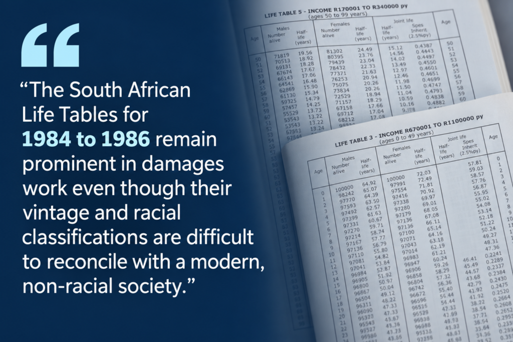
The South African Life Tables for 1984 to 1986 remain prominent in damages work even though their vintage and racial classifications are difficult to reconcile with a modern, non-racial society.
The six tables reproduced in the Quantum Yearbook materials attempt to classify mortality by annual earnings. Their structure is set out below. The historical labels in quotation marks identify the source tables – they do not imply endorsement of those categories.
Six income related mortality bases reproduced in the supplied Quantum Yearbook materials
| Table | Annual earnings band | Mortality basis |
|---|---|---|
| 1 | More than R1 600 000 | 80% of SALT 1984 to 1986 "White" mortality |
| 2 | R1 100 001 to R1 600 000 | 100% of SALT 1984 to 1986 "White" mortality |
| 3 | R670 001 to R1 100 000 | 67% "White" plus 33% "Coloured" mortality |
| 4 | R340 001 to R670 000 | 33% "White" plus 67% "Coloured" mortality |
| 5 | R170 001 to R340 000 | 100% of SALT 1984 to 1986 "Coloured" mortality |
| 6 | Less than R170 001 | 120% of SALT 1984 to 1986 "Coloured" mortality |
Important limitation These are not six independently observed modern population tables. They are blends or adjustments of two legacy mortality bases. Income changes the selection rule, but it does not create new underlying mortality observations.
Income is a proxy and not proof
Income is relevant in life expectancy calculations because mortality and socio-economic conditions are associated.
It is nevertheless a proxy.
An annual earnings figure does not directly measure education, occupation, housing, geography, access to healthcare, smoking, body mass, co-morbidity or the other factors that may affect longevity. Nor does it establish how those factors interact for the person before the court.
Also, mechanical use of an income band creates further questions.
Which income are we referring to: pre-accident earnings, income at the valuation date, or the career path projected but for the injury?
How should the table be chosen for a child, a student, a temporarily unemployed claimant, a homemaker or a person whose earnings fluctuate?
What happens when projected income crosses several bands during the working lifetime?
A banded system also creates cliff effects. A small difference in assumed annual income can switch the entire mortality table even though the underlying evidence about the person’s longevity has barely changed. If the bands are stated in nominal rand, their date and inflation policy matter. Without regular re-basing, inflation alone will move claimants into lighter mortality categories.
These concerns do not make income irrelevant. They make the reasoning visible. A defensible selection should explain why the chosen proxy is appropriate and should test another basis where the classification is uncertain or the amount is sensitive.
What the courts have established
• Singh and Another v Ebrahim (413/09) [2010] ZASCA 145, especially paragraphs 13 to 22, 65, 151 to 168 and 199, is the leading South African decision on life expectancy evidence in a damages claim.
The case concerned a severely disabled child and divided the Supreme Court of Appeal on the ultimate result.
On the mortality table issue, however, both the majority and dissent accepted use of the 1984 to 1986 table on the evidence before the court. The dissent described the attempt to relate mortality to income as attractive in principle, but found that the evidence did not establish the reliability of the income classifications.
Singh should not be read as freezing mortality science in 2010. The court’s conclusion was evidentiary: the older table was the best available basis proved in that case.
Later decisions, including AD and Another v MEC for Health and Social Development Western Cape [2016] ZAWCHC 116, and PM obo TM v MEC for Health Gauteng [2017] ZAGPJHC 346, followed the established tables where a better basis had not been proved.
The practical lesson is demanding but constructive. A departure needs evidence, a reproducible method and reasons. Novelty alone is not enough, but neither is habit.
Singh also explains the proper relationship between group data and individual evidence. A mortality table starts with a sufficiently similar group and its annual death rates. Medical evidence then identifies claimant-specific features that may justify an adjustment. The court must decide the facts and probabilities, the actuary should show how those findings change the calculation.
An unexplained round deduction or unexplained departure from an expert’s survival estimate weakens the chain of reasoning.
Three questions that should not be collapsed
Disputes become confused when baseline mortality, medical impairment and general contingency are treated as interchangeable.
They answer different questions and rely on different evidence.
Distinct layers in a mortality informed damages calculation
| Layer | Question | Primary evidence | Role in calculation |
|---|---|---|---|
| Baseline mortality | Which population mortality curve is the starting point | Actuarial and demographic evidence | Annual survival probabilities |
| Claimant specific adjustment | How an injury or condition changes mortality relative to the baseline | Medical evidence interpreted in an actuarial model | Adjusted mortality curve or survival distribution |
| Other future uncertainty | What non-mortality risks affect earnings, support or expenditure | Factual, labour market and legal evidence | Contingency or scenario adjustment |
Keeping the layers separate guards against double counting. If a medical condition has already increased the mortality rates in the survival curve, a further contingency for the same shortened life risk requires a distinct justification.
The same caution applies when a court or expert truncates the period of future loss at a stated life expectancy and also applies annual survival probabilities. A mean lifetime should not become a hard cut-off unless the model and evidence expressly support that treatment.
The result can move materially
Vector Actuaries re-ran six completed loss of earnings calculations using each of the six tables in the supplied framework. Every other assumption was held constant. The matters below are anonymised.
The comparison is a sensitivity analysis, not a claim that Table 1 or Table 6 is correct for any claimant.
Interactive sensitivity analysis
How much can the life table change the result?
Select an anonymised matter to see what happened when the same loss-of-earnings calculation was run using Table 1 and Table 6. Every other assumption was held constant.
Mr Tshimbiluni
Male aged 29Difference in calculated loss
Table 1 compared with Table 6
What this shows: The percentage effect is not ordered neatly by age. It also depends on the timing and shape of the projected loss, retirement assumptions and the relationship between the uninjured and injured earnings paths.
How to read this: The percentage is measured against the Table 6 result. These six matters are illustrative and do not form a representative statistical sample. The comparison demonstrates sensitivity; it does not establish which table is appropriate for a particular claimant.
The effect differs by head of damage
Loss of earnings
Survival probabilities weight both the uninjured and injured earnings streams. The effect on the final loss depends on the difference between those streams in each year, not simply on the claimant’s total prospective earnings. A late-career promotion, an altered retirement assumption or a post-injury residual earning capacity can materially change how the mortality basis operates.
Loss of support
The calculation may involve the survival of the deceased but for the death, the survival of each dependant, the duration of dependency and the way family income would have been shared.
Joint survival probabilities may be required. The same mortality assumption can also affect questions about accelerated benefits or inheritance, which should be modelled consistently rather than handled through an unexplained deduction.
Future medical and care costs
Future treatment, equipment, therapy and care costs are incurred only while the claimant is alive, subject to the evidence about their timing.
A reduced life expectancy can therefore reduce a large care award. That makes the conversion of medical opinion into an annual survival curve especially important. A clinician may estimate relative risk, a range of survival or a mean remaining lifetime; those statements are not mathematically interchangeable.
A life table has two clocks
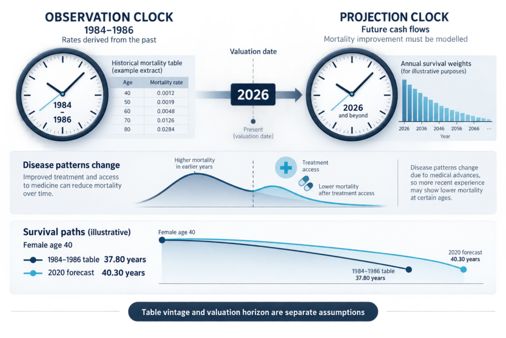
The first clock is the observation period from which mortality rates were derived. The second is the future period over which the claimant’s cash flows are projected. A 1984 to 1986 table applied to a young claimant in 2026 may weight payments many decades after the data period. If mortality improves over time, a static period table will not capture that improvement unless the model makes an explicit projection.
Whittaker’s 2021 analysis illustrates the issue. His forecast tables produced longer remaining lifetimes than the 1984 to 1986 tables at many ages. For a female aged 40, the paper reports 37.80 remaining years under the older table and 40.30 under the 2020 forecast. The point is not that the forecast must replace the established basis in every case. It is that table vintage, mortality improvement and the valuation horizon are separate assumptions that should be disclosed.
Disease patterns also change. South Africa’s HIV mortality experience was transformed by access to antiretroviral treatment. A population table containing a historical HIV-related mortality hump may not represent a claimant whose diagnosis, treatment and adherence are known. Conversely, a general improvement assumption cannot substitute for medical evidence about a specific person.
The actuary needs a defensible baseline, while the medical experts need to address the claimant-specific departure from it.
What a defensible actuarial report should disclose
A legal reader should not have to infer the mortality model from a final capital value. At minimum, the report should make the following matters traceable.
- The table and version Name the source, data period, sex basis, adjustment or blend, and any mortality improvement assumption.
- The selection reason Connect the chosen basis to admissible facts about the claimant. If income bands are used, identify the earnings measure, date and band.
- The calculation method Confirm that annual survival probabilities were applied and explain any joint-life or dependant-life modelling.
- Medical adjustments State which medical findings change mortality, how they were converted into the curve, and whether a range was supplied.
- Limitations Identify gaps in the demographic or medical evidence and distinguish actuarial assumptions from facts found by the court.
Questions attorneys should ask
The following questions are suitable for instructions, expert conferences and cross-examination.
- Which life table was used, and where can the underlying annual mortality rates be found?
- Why is that population a reasonable baseline for this claimant?
- If the choice depends on income, which income measure and date were used, and why?
- Were there any adjustments made to the base table?
- If so, which parts of the adjustment come from medical experts, and which are actuarial judgement?
- How does the result change under the strongest reasonable alternative basis?
- Would the table choice affect other heads of damage or accelerated benefits in the same matter?
The table should be evidence rather than habit
Life tables are indispensable because courts must value uncertain future cash flows. They do not remove uncertainty. They organise it. The apparent precision of a capital value depends on the quality of the population data, the fit between that population and the claimant, the medical evidence and the transparency of the model.
South African practice faces a genuine difficulty: the established complete tables are old and historically classified, while proposed alternatives have not always been supported by evidence strong enough to satisfy the courts. That tension should produce better disclosure and testing, not automatic loyalty to either the oldest or the newest source.
For attorneys, the practical safeguard is simple. Understand which table was used and why.
A mortality assumption capable of moving a damages calculation by hundreds of thousands of rand belongs in the contested reasoning of the case, not in the small print of an actuarial report.
The central point – A damages figure can look precise while concealing a contestable mortality assumption. The selected life table determines the probability attached to every future year of earnings, support or care. In six illustrative loss of earnings matters, changing only that table moved the calculated loss by 7.9% to 18.6%.
That result does not prove that the lightest mortality table is correct, or that the heaviest one is. It shows that table selection is material evidence. An attorney should be able to identify the mortality basis, understand why it fits the claimant, and test what happens if a reasonable alternative is used.